주식 데이터 시각화

따릉이 프로젝트를 마친 민서에게 선배가 새로운 도전을 제안했습니다. "주식 데이터도 한번 다뤄봐. 시계열 데이터 다루는 법이랑 수익률 분석은 어디서든 써먹거든."

민서는 처음에 "주식은 잘 모르는데"라고 했지만, 선배가 말했습니다. "주식을 몰라도 돼. 숫자 패턴을 읽는 거야."

프로젝트 개요

분석 주제: 주요 기업 주가 데이터 비교 분석

분석 질문

• 기업별 주가는 어떤 추이를 보이는가.
• 일별 수익률 분포는 어떤 모양인가.
• 기업들 사이에 수익률 상관관계가 있는가.
• 거래량과 가격 변화 사이에 관계가 있는가.

1단계: 샘플 주식 데이터 생성

import pandas as pdimport numpy as npimport seaborn as snsimport matplotlib.pyplot as pltnp.random.seed(42)# 2023년 영업일 기준 날짜 생성dates = pd.bdate_range(start="2023-01-02", end="2023-12-29")n_days = len(dates)companies = {    "TechA": {"start": 50000, "mu": 0.0008, "sigma": 0.018},    "TechB": {"start": 80000, "mu": 0.0005, "sigma": 0.022},    "FinanceC": {"start": 30000, "mu": 0.0003, "sigma": 0.012},    "RetailD": {"start": 15000, "mu": 0.0001, "sigma": 0.015},}# 기하 브라운 운동(GBM)으로 주가 시뮬레이션price_data = {}volume_data = {}for name, params in companies.items():    # 일별 수익률 생성 (정규분포)    daily_returns = np.random.normal(        params["mu"], params["sigma"], n_days    )    # 누적 곱으로 주가 경로 생성    price_path = params["start"] * np.cumprod(1 + daily_returns)    price_data[name] = price_path.round(0).astype(int)    # 거래량: 가격 변동이 클수록 거래량 증가    base_volume = np.random.lognormal(mean=10, sigma=0.5, size=n_days)    volume_shock = np.abs(daily_returns) / params["sigma"]    volume_data[name] = (base_volume * (1 + volume_shock)).astype(int)# 종가 DataFrameprice_df = pd.DataFrame(price_data, index=dates)price_df.index.name = "date"# 거래량 DataFramevolume_df = pd.DataFrame(volume_data, index=dates)volume_df.index.name = "date"print("=== 주가 데이터 (wide-form) ===")print(price_df.head())print(f"\n크기: {price_df.shape}")print(f"\n기본 통계:")print(price_df.describe().round(0))

2단계: long-form 변환 및 수익률 계산

# wide-form → long-form 변환price_long = price_df.reset_index().melt(    id_vars="date",    var_name="company",    value_name="close")# 일별 수익률 계산 (회사별로 pct_change 적용)price_df_copy = price_df.copy()return_df = price_df_copy.pct_change().dropna()return_df.index.name = "date"return_long = return_df.reset_index().melt(    id_vars="date",    var_name="company",    value_name="return")# 거래량도 long-form으로volume_long = volume_df.reset_index().melt(    id_vars="date",    var_name="company",    value_name="volume")# 통합 DataFramefull_df = price_long.merge(return_long, on=["date", "company"])full_df = full_df.merge(volume_long, on=["date", "company"])full_df["return_pct"] = full_df["return"] * 100print("=== 통합 데이터 (long-form) ===")print(full_df.head(8))print(f"\n크기: {full_df.shape}")

3단계: 종가 추이 (lineplot)

plt.figure(figsize=(12, 5))# 회사별로 시작가를 1로 정규화하여 상대 비교normalized = price_df.div(price_df.iloc[0])normalized_long = normalized.reset_index().melt(    id_vars="date",    var_name="company",    value_name="normalized_price")sns.lineplot(    data=normalized_long,    x="date",    y="normalized_price",    hue="company",    linewidth=1.5)plt.axhline(y=1.0, color="black", linestyle="--", linewidth=0.8, alpha=0.5)plt.title("Normalized Stock Price Trend (Base = 1.0 at Start)")plt.xlabel("Date")plt.ylabel("Normalized Price")plt.legend(title="Company")plt.tight_layout()plt.show()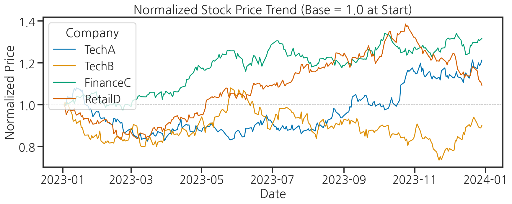

4단계: 일별 수익률 분포 (histplot + kdeplot)

fig, axes = plt.subplots(2, 2, figsize=(12, 8))axes = axes.flatten()companies_list = list(companies.keys())colors = sns.color_palette("Set2", 4)for i, (company, color) in enumerate(zip(companies_list, colors)):    company_returns = return_df[company] * 100    # 히스토그램 + KDE    sns.histplot(        data=company_returns,        bins=40,        kde=True,        color=color,        alpha=0.7,        ax=axes[i]    )    # 평균선과 0선 추가    axes[i].axvline(x=0, color="black", linestyle="--",                    linewidth=1, alpha=0.7)    axes[i].axvline(x=company_returns.mean(), color="red",                    linestyle="-", linewidth=1.5, label=f"Mean: {company_returns.mean():.3f}%")    axes[i].set_title(f"{company} Daily Returns")    axes[i].set_xlabel("Daily Return (%)")    axes[i].set_ylabel("Count")    axes[i].legend(fontsize=9)plt.suptitle("Distribution of Daily Returns by Company", fontsize=13)plt.tight_layout()plt.show()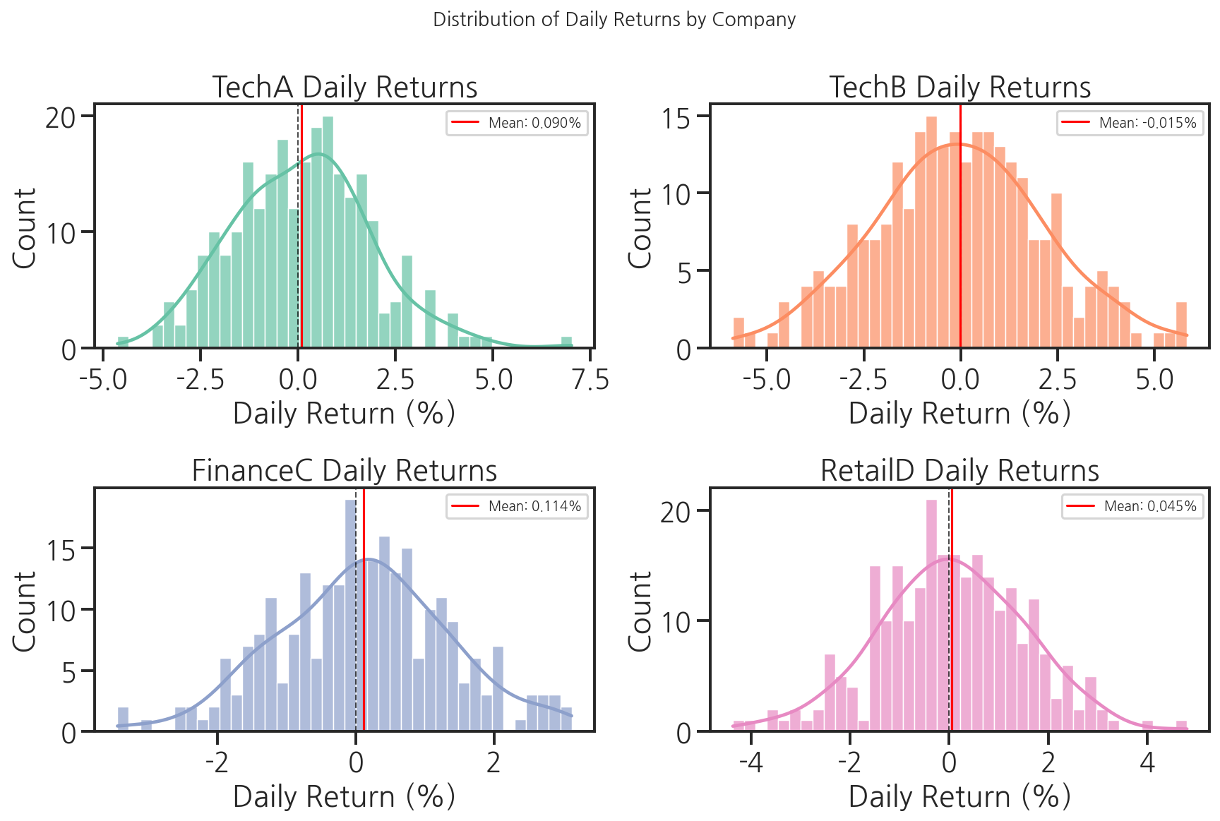

5단계: 수익률 상관관계 (heatmap)

# 수익률 상관행렬 계산corr_matrix = return_df.corr().round(3)print("수익률 상관행렬:")print(corr_matrix)plt.figure(figsize=(7, 6))sns.heatmap(    corr_matrix,    annot=True,    fmt=".3f",    cmap="coolwarm",    center=0,    vmin=-1,    vmax=1,    linewidths=0.5,    cbar_kws={"label": "Correlation"})plt.title("Return Correlation Matrix")plt.tight_layout()plt.show()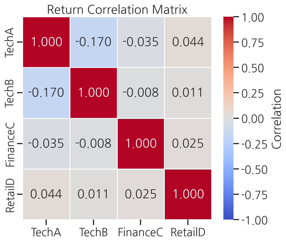

6단계: 거래량과 가격 변화 관계 (regplot)

# TechA의 거래량(log)과 절대 수익률 관계tech_a = full_df[full_df["company"] == "TechA"].copy()tech_a = tech_a.dropna(subset=["return"])tech_a["abs_return_pct"] = tech_a["return_pct"].abs()tech_a["log_volume"] = np.log10(tech_a["volume"])plt.figure(figsize=(8, 5))sns.regplot(    data=tech_a,    x="log_volume",    y="abs_return_pct",    scatter_kws={"alpha": 0.3, "s": 15},    line_kws={"color": "red", "linewidth": 2})plt.title("TechA: Log Volume vs Absolute Daily Return")plt.xlabel("Log10(Volume)")plt.ylabel("Absolute Return (%)")plt.tight_layout()plt.show()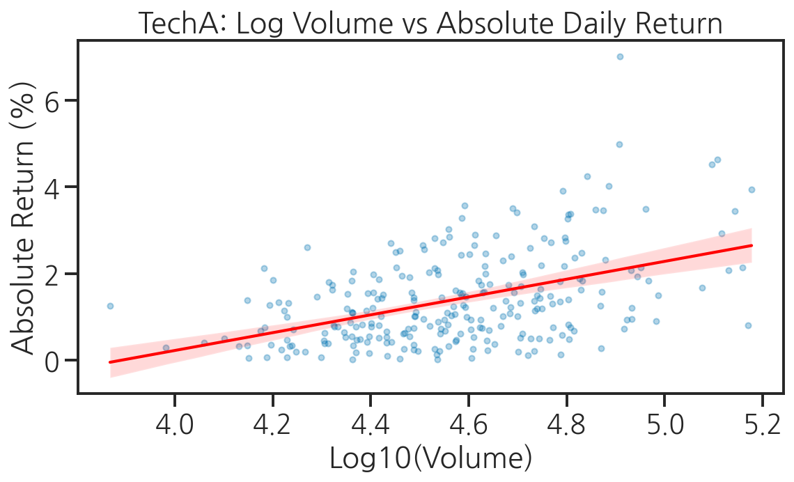

7단계: 기업별 수익률 비교 (violinplot)

plt.figure(figsize=(10, 5))sns.violinplot(    data=return_long,    x="company",    y="return",    hue="company",    palette="Set2",    inner="quartile",   # 사분위수 표시    legend=False)plt.axhline(y=0, color="black", linestyle="--", linewidth=1, alpha=0.7)plt.title("Daily Return Distribution by Company (Violin Plot)")plt.xlabel("Company")plt.ylabel("Daily Return")plt.tight_layout()plt.show()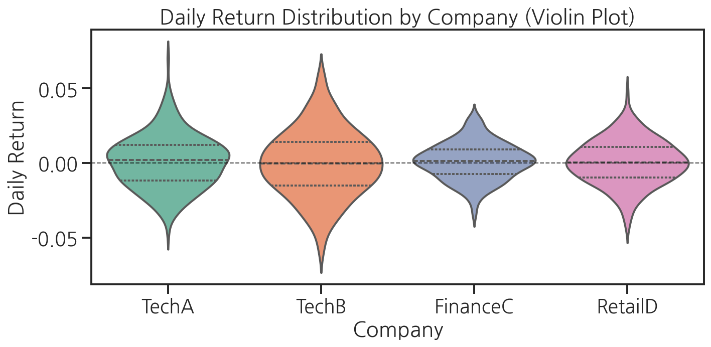

8단계: pairplot으로 전체 관계 요약

# 월별 집계로 pairplot용 데이터 준비monthly_stats = []for company in companies_list:    company_data = full_df[full_df["company"] == company].copy()    company_data["month"] = pd.to_datetime(company_data["date"]).dt.month    monthly = company_data.groupby("month").agg(        avg_close=("close", "mean"),        avg_return=("return_pct", "mean"),        volatility=("return_pct", "std"),        avg_volume=("volume", "mean")    ).reset_index()    monthly["company"] = company    monthly_stats.append(monthly)monthly_df = pd.concat(monthly_stats, ignore_index=True)# pairplotg = sns.pairplot(    monthly_df[["avg_close", "avg_return", "volatility", "avg_volume", "company"]],    hue="company",    palette="Set2",    plot_kws={"alpha": 0.7},    diag_kind="kde")g.figure.suptitle("Pairplot: Monthly Statistics by Company", y=1.02)plt.tight_layout()plt.show()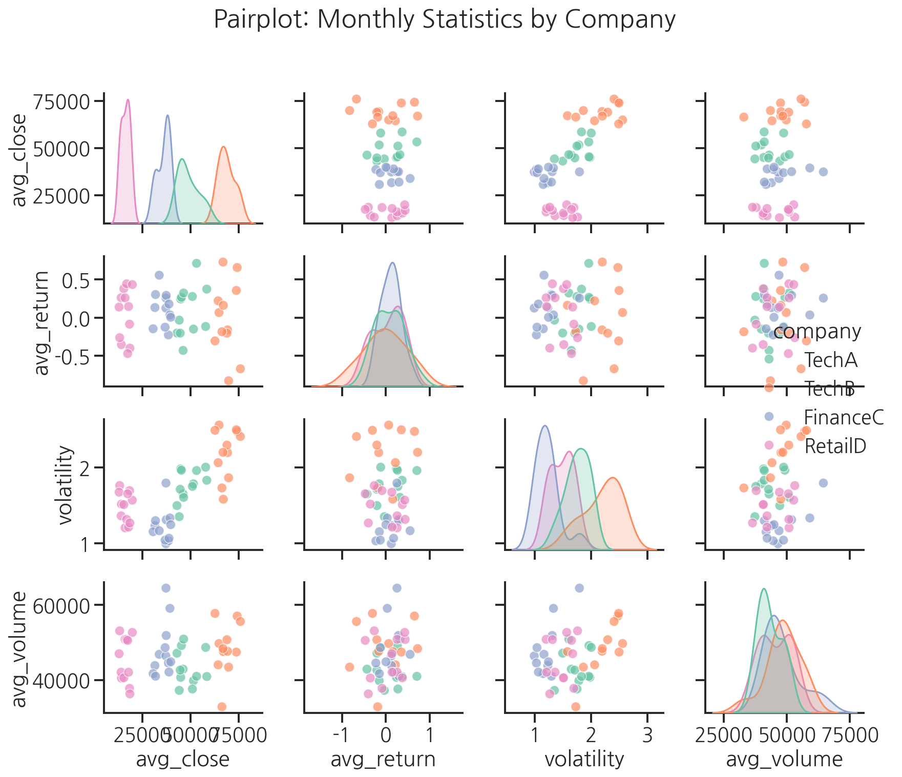

결과 저장 및 해석

# 최종 요약 대시보드 저장fig, axes = plt.subplots(2, 2, figsize=(14, 10))fig.suptitle("Stock Analysis Dashboard (2023)", fontsize=14, fontweight="bold")# (0, 0) 정규화 주가 추이normalized_long_plot = normalized.reset_index().melt(    id_vars="date", var_name="company", value_name="norm_price")sns.lineplot(data=normalized_long_plot, x="date", y="norm_price",             hue="company", linewidth=1.5, ax=axes[0, 0])axes[0, 0].axhline(y=1.0, color="black", linestyle="--", linewidth=0.8, alpha=0.5)axes[0, 0].set_title("Normalized Price Trend")axes[0, 0].set_xlabel("")axes[0, 0].set_ylabel("Normalized Price")axes[0, 0].legend(title="Company", fontsize=8)# (0, 1) 수익률 분포 (violinplot)sns.violinplot(data=return_long, x="company", y="return",               hue="company", palette="Set2",               inner="quartile", legend=False, ax=axes[0, 1])axes[0, 1].axhline(y=0, color="black", linestyle="--", linewidth=1, alpha=0.7)axes[0, 1].set_title("Return Distribution")axes[0, 1].set_xlabel("Company")axes[0, 1].set_ylabel("Daily Return")# (1, 0) 상관행렬 heatmapsns.heatmap(corr_matrix, annot=True, fmt=".2f", cmap="coolwarm",            center=0, ax=axes[1, 0], cbar_kws={"shrink": 0.8})axes[1, 0].set_title("Return Correlation")# (1, 1) 월별 변동성volatility_monthly = return_long.copy()volatility_monthly["month"] = pd.to_datetime(volatility_monthly["date"]).dt.monthvol_pivot = volatility_monthly.groupby(["month", "company"])["return"].std().reset_index()vol_pivot.columns = ["month", "company", "volatility"]sns.lineplot(data=vol_pivot, x="month", y="volatility",             hue="company", marker="o", ax=axes[1, 1])axes[1, 1].set_title("Monthly Volatility")axes[1, 1].set_xlabel("Month")axes[1, 1].set_ylabel("Std of Daily Returns")axes[1, 1].legend(title="Company", fontsize=8)plt.tight_layout()plt.savefig("stock_dashboard.png", dpi=150, bbox_inches="tight")print("대시보드 저장 완료: stock_dashboard.png")plt.show()# 핵심 인사이트 출력print("\n=== 분석 결과 요약 ===")for company in companies_list:    returns = return_df[company] * 100    total_return = (price_df[company].iloc[-1] / price_df[company].iloc[0] - 1) * 100    print(f"{company}: 연간 수익률 {total_return:.1f}%, "          f"평균 일변동 ±{returns.std():.2f}%")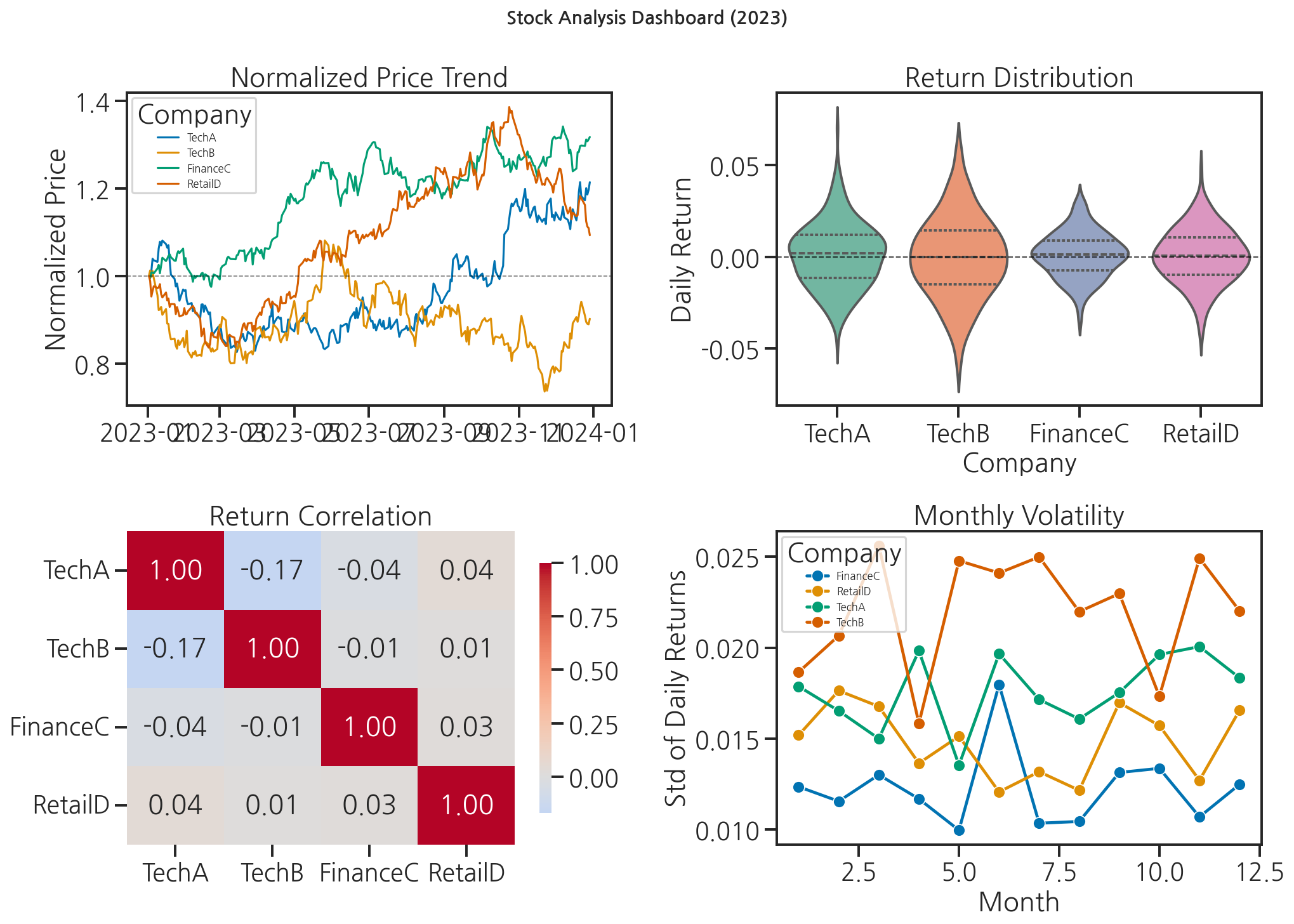

"선배, 이거 보니까 TechB가 변동성이 제일 크네요." 민서가 말했습니다. "변동성이 크다는 게 위험하다는 건데, 그걸 숫자로만 보면 실감이 안 나는데 바이올린 플롯으로 보니까 확 와닿아요."

선배가 고개를 끄덕였습니다. "그게 시각화의 힘이야."

핵심 정리

• 시계열 데이터는 wide-form으로 저장하고, Seaborn 시각화를 위해 long-form으로 변환합니다.
• 절대 주가 대신 정규화된 가격을 사용하면 여러 기업을 공정하게 비교할 수 있습니다.
• corr()과 heatmap으로 변수 간 상관관계를 한눈에 파악합니다.
• pairplot은 여러 변수 쌍의 관계를 한번에 탐색하는 강력한 도구입니다.
• 분석 마지막에는 반드시 숫자 요약과 함께 인사이트를 문장으로 정리합니다.